
Course 1: Modeling Linear Programming
Author: OptimizationCity Group
What is Operations Research?
Operations research is a scientific approach to the decisions that are made during the operation of organized systems. In other words, operations research is used in issues related to the guidance and coordination of operations and various activities. Operations research is used in a variety of fields such as economics, trade, industry, government, health, and so on. Operations research examines issues with a systematic approach and tries to resolve the conflict of resources between different parts of an organization in such a way that the best result or the optimal answer is created for the whole organization.
Operations research includes various sections, of which mathematical linear programming is one of the most important. In linear programming, a mathematical model is used to explain the problem. The word linear means that all mathematical relations of this model must necessarily be linear. The birth of linear programming dates back to 1947, when George Dantzig invented the simplex method for solving general linear programming problems for the optimal programming computation project. The invention was so influential in management science that it led George Dantzig to the Nobel Prize but never won it.
Formulating the problem in the form of linear programming
We continue this section by formulating a small example of linear programming. This example is simple enough that it can be studied graphically.
Example: A door and window manufacturing company has three plants. plant 1 produces aluminum frames and metal parts. In plant 2, wooden frames are produced; and in plant 3, the glass is cut and mounted on the frames. The manager of these workshops is looking to produce two new products. He/she has asked the operations research center to increase the production of each product according to the capacity of the plants. Product 1 is a door with an aluminum frame and product 2 is glass windows with a wooden frame. Due to the fact that both products require plant 3 for welding, the capacity of this plant will lead the competition between these two products. The table below shows all data you need.
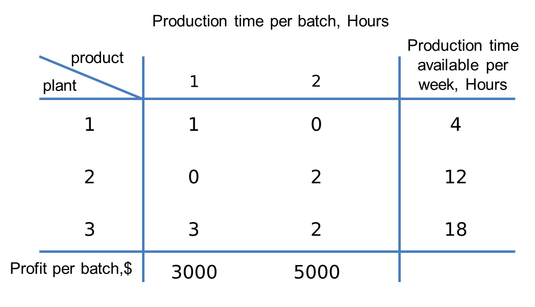
x1 and x2 represent the number of products 1 and 2 per hours, respectively, and z represents the profit from sales per hour. In the operations research literature, x1 and x2 are called decision variables and z is called an objective function.
To produce each unit of product 1, 1 unit of plant 1 is used, which has only 4 units of capacity for the new product per hour of plant 1. This constraint is displayed algebraically x1≤4. Similarly for plant 2, a limit 2x2≤12 is required for Product 2. plant 3 capacity is used by both products, which limits 3x1 +2x2≤18. Because products cannot be negative, the decision variables are non-negative, and its mathematical representation is x1≥0, x2≥0. The mathematical representation of the linear programming model is summarized as follows.

Because this linear programming model consists of only two variables x1 and x2, a graphic method can be used to solve the linear program. This method requires drawing a shape with axes x1 and x2. Each constraint covers a part of the two-dimensional axis, which creates a feasible region from sharing these constraints. We are looking for the point that creates the maximum value of the objective function, z. To draw the feasible region, we add the constraints one by one as follows.

Note: To add the constraint 3x1+2x2<=18 to the feasible region, it is enough to draw the equation 3x1+2x2=18 first. Given that the point of the origin (x1=0,x2=0) holds in the constraint, the space below the line of equation shows the 3x1+2x2<=18. The only remaining step is to find the point that maximizes the value in the area.
Suppose that Z=10. If this value is within the feasible region, this value can be increased. Otherwise it must be decreased to be in the feasible region. By increasing the value by 10 to 20, the line would be still in the feasible region. In this way, by increasing the constant value(C) of the line C=3x1+5x2, a set of particular parallel lines is drawn, and finally the line that has the greatest distance with the origin is selected. As shown in the figure below, point (2,6) crosses the line 3x1+5x2=36 and this point (x1=2,x2=6) generates the most revenue for the workshop. Therefore, by producing 2 units of product 1 and 6 units of product 2, the most revenue (36) per minute is generated.

Mathematical representation of linear model
In this section, the problem of door and window manufacturing company can be generalized. In this problem, there are 3 plants or resources with limited capacity that two products should use three resources according to their needs.
In the general form, suppose that we want to assign m sources to n competing products. Assume that xj is the amount of product j and Z are the measure of efficiency want to be maximize. Also assume that cj is the change of Z is due to each unit of increase xj , bi is the amount of source i, and aij is the amount of source i consumed by the product j. A summary of the information is given in the table below.

According to the table above, the general form resource allocation problem can be expressed in mathematical form as follows.

The above standard model is called the linear programming problem.
Terms of linear programming model
For simplicity in expressing problems in linear programming, common words are defined as follows.
Objective function: Refers to the function c1x1+c2x2+…+cnxn that is intended to find the maximum.
Functional constraint: refers to a function that indicates the total consumption of each resource for all products.
Non-negativity constraint: Refers to xj>=0
Constraint: Refers to the set of functional constraints and Non-negativity.
Decision variable: Refers to the variable xj that indicate the amount of each product.
Parameter: Refers to data aij,bi,cj
Note: The standard model may differ from linear programming models in reality. Other forms of linear programming problem that can be converted to standard form are as follows:
- Instead of maximizing (Max), minimizing (Min) may be considered.
- Some functional constraints may be greater than equal(>= ):
![]()
- Some functional constraints may be equal:
![]()
Some variables may be only negative; or either negative or positive (unrestricted in sign).
Term of linear program solution
Solution: Refers to any set of values assigned to decision variables (x1,x2,…,xn). For example, in the previous example, points (2,3) and (5,5) are the answers of the linear programming model, and it does not matter if they are inside or outside the feasible region.

Feasible solution: Refers to the solution that applies to all constraints (functional and non-negative). For example, in the figure above, point (2,3) is a feasible solution and solution (5,5) is an infeasible solution.

Optimal solution: A feasible solution for which the value of the objective function is the most desirable. The following figure shows the optimal solution to the previous example.

There are four possibilities for the optimal solution:
1- Unique optimal solution: In this case, the optimal solution is only one point of feasible region (similar to the figure above).
2- Multiple (alternative) optimal solution: Often the linear programming problem has a single solution. But this is not necessarily the case. In the previous example, if the profitability of product 2 decreases from 5 to 2 units, then the line of the objective function will be parallel to the line , and therefore all points on the line between points (2,6) and (4,3) are the optimal solution.

3-Unbound solution: This solution occurs when the constraints can not prevent the infinite increase of the objective function (Z) in the desired direction. In the previous example, if both constraints 2x2<=12 and 3x1+2x2<=18 are omitted, the possible space becomes as follows where the value of the objective function can be increased infinitely.

4- Infeasible solution: In this case, the problem has no feasible solution or the feasible region is empty. In the previous example, if the constraint 2x2<=12 changes to 2x2>=12 and the constraint x1<=4 changes to x1>=4, the feasible region is empty and the problem has no solution..
5- Degeneracy
In a two-variable problem, if there is a corner point of the intersection of more than two constraints, it is a degeneracy problem (this problem can be used for n-variable problems). To clarify the issue, consider the following example:
Example: Consider this problem:

Its graphical representation is as follows.

In this problem, it can be seen that at point A, three corner points have coincided. The points are:
1) The point resulting from the intersection of the constraints corresponding to the first constraint with the x2 axis
2) The point resulting from the intersection of the constriants corresponding to the second constraint with the x2 axis
3) The point resulting from the intersection of the constraints corresponding to both constraints
Later, it is said that in the simplex method, each iteration actually represents the characteristics of a corner point, and since several corner points coincide in degeneracy, we may encounter a situation where in successive iterations on these points.
Classification of linear programming
In the previous parts, special cases of linear programming problems were stated. In a general classification, the types of possible situations for the optimal solution of linear programming are as follows.

The types of possible cases that can occur in the feasible region of a bivariate linear programming model are shown in the figure below.

Classification of constraints in linear programming
According to the effect of the constraint on the formation of the feasible region and how the optimal solution is found on them, the constraints can be classified into two groups.
Effective constraints
There are constraints that are effective in forming the feasbile area, and adding any new effective limitation to the model causes a decrease in the justified area, and removing the effective restriction causes an increase in the justified area.
Redundant constraints
There are restrictions that do not affect the creation of the feasbile area, and their presence or absence does not change the feasbile area.
Example: Consider this problem.

The graphical representation of this problem is as follows.

Note that only the first constraint and the non-negativity constraints are involved in forming the feasbile region. The second and third constraints have no role in creating the feasible region and determining the optimal solution. These two restrictions are redunfant constriants.
Example: An area consists of three farms with two limitations, land and water, that limit the possibilities of planting these farms. Information on the water alocation and usable land of the three farms is given in the table below.

The crops suited for this region include sugar beets, cotton, and sorghum. These crops differ primarily in their expected net return (profit) per acre and their consumption of water. In addition, the maximum acreage that can be devoted to each of these crops is set.


To ensure equity between the three farms, it has been agreed that every famer will plant the same proportion of its available land. For example, if farm 1 plants 200 of its available 400 acres, then farm 2 must plant 300 of its 600 acres, while farm 3 plants 150 acres of its 300 acres. However, any combination of the crops may be grown at any of the farm.
The job is to plan how many acres to devote to each crop at the farms while satisfying the given restrictions. The objective is to maximize the total net return as a whole.
Solution: We are going to formalate this problem as a linear programming model. The quantities to be decided are the number of acres to devote to each of the three crops at each of the three farms, which are the decision variables as follows.

For example, in the above table, means the area of farm 1 in acre to devote the suger beets. Since the objective function Z is the total net return, the resulting linear programming model for this problem is:
Max Z=400(x1+x2+x3)+300(x4+x5+x6)+100(x7+x8+x9)
Subject to the following constraints:
1) Usable land for each farm(acre):
Farm 1: x1+x4+x7<=400
Farm 2:x2+x5+x8<=600
Farm 3:x3+x6+x9<=300
2) Water allocation for each farm:
Farm 1: 3x1+2x4+x7<=600
Farm 2: 3x2+2x5+x8<=800
Farm 3: 3x3+2x6+x9<=375
3) Total acreage for each crop:
Crop 1:x1+x2+x3<=600
Crop 2:x4+x5+x6<=500
Crop 3:x7+x8+x9<=325
4) Equal proportion of land planted:
Equality of cultivated land to usable land for farms 1 and 2:
(x1+x4+x7)÷400=(x2+x5+x8)÷600
Equality of cultivated land to usable land for farms 1 and 3:
(x1+x4+x7)÷400=(x3+x6+x9)÷300
Equality of cultivated land to usable land for farms 2 and 3:
(x2+x5+x8)÷600=(x3+x6+x9)÷300
The above equations are not yet in an appropriate form for a linear programming model because some of the variables are on the right-hand side. Hence, their final form is:
3(x1+x4+x7)-2(x2+x5+x8)=0
4(x3+x6+x9)-3(x1+x4+x7)=0
(x2+x5+x8)-2(x3+x6+x9)=0
5) Non-negativity of decision variables is as follows.
xj>=0 for all j=1,…,9
The optimal solution to the above linear programming model is as follows:

Example: The financial manager of a company is responsible for investing 10 million dollar in stock market. She can also use 1 million dollar loan with a 5.5% interest rate before tax. The type, their quality rating, expiration time and rate of return are listed in the below table.

There are the following limitations on investment:
- The total investment in type of government and cooperation should be at least $ 4 million
- The average quality scale should not exceed 1.4(note that the smaller number means the higher quality).
- The average duration of validity should not exceed 5 years.
Assuming that the stock manageris going to maximize returns after tax (at the rate of 50% and miniucipility is tax-exempt). which type of investment should she buy? Is borrowing up to $ 1 million recommended (interest rate for taking load after tax is 2.75%)?
Solution: The amount of investment in each type and the amount of the loan are the decision variables expressed as follows.
xA: The amount of investment in type A in millions of dollars
xB: The amount of investment in type B in millions of dollars
xC: The amount of investment in type C in millions of dollars
xD: The amount of investment in type D in millions of dollars
xE: The amount of investment in type E in millions of dollars
Y: Loan amount with interest rate of 5.5% before tax in millions of dollars
Total income after tax (assuming 50% tax and miniucipility type being tax-exempt) is as follows:
Z=0.043xA+0.027xB+0.025xC+0.022xD+0.045xE-0.0275Y
The constsraints are as follows:
- The manager can only invest $10 million to which the loan amount Y is added:
xA+xB+xC+xD+xE<=10+Y
- The manager should invest at least $4 million in the purchase of cooperation(xB) and government(xC,xD):
xB+xC+xD>=4
- The quality to the total investment should not exceed 1.4. Note that the smaller value means the higher quality:
(2xA+2xB+xC+xD+5xE)÷(xA+xB+xC+xD+xE)<=1.4
- Multiplying the denominator (xA+xB+xC+xD+xE) on both sides results in the following:
0.6xA+0.6xB-0.4xC-0.4xD+3.6xE<=0
- The average duration of validity should not exceed 5 years, which is expressed as follows:
(9xA+15xB+4xC+3xD+2xE)÷(xA+xB+xC+xD+xE)<=5
- Multiplying the denominator on both sides gives the following:
4xA+10xB-xC-2xD-3xE<=0
- The maximum loan is $1 million, which is included in the model as a following limitation:
Y<=1
- Non-negativity of decision variables are as follows:
xA,xB,xC,xD,xE,Y>=0
The optimal solution to the above linear programming model is as follows:

Example: A Company has discontinued the production of a certain unprofitable product line, which creating the excess capacity on machines. The management is considering devoting this excess capacity to products; products 1, 2, and 3. The available capacity on the machines is summarized in the following table:


The number of machine-hour required for each unit of the products is:

The sales department indicates that the sales potential for products 1 and 2 exceeds the maximum production rate and the sales potential for product 3 is 20 units per week. The unit profit would be $50, $20, and $25, respectively, on products 1, 2, and 3. The objective is to determine how much of each product should produce to maximize profit. Formulate a linear programming model for this problem.
Solution:
Let be the number of units of product i produced for i=1,2,3. The linear programming model of this problem is as follows.

Constraint 1 is the same as milling machine capacity, constraint 2 is the same as lather machine capacity, constraint 3 is the same as grinder machine capacity, and constraint 4 is demand constriant.
The optimal solution to the above linear programming model is as follows:

Example: Consider the following problem, where the value of c1 has not yet been certain.

Use graphical analysis to determine the optimal solution(s) for (x1, x2) for the various possible values of c1.
Solution:


Example: The Company produces precision medical equipment at two factories. Three medical customers have placed orders for products. The table below shows what the cost would be for shipping each unit from each factory to each of these customers. Also shown are the number of units that will be produced at each factory and the number of units ordered by each customer.

A decision now needs to be made about the shipping plan for how many units to ship from each factory to each customer.
Solution:
Let xij be the number of units shipped from factory i (1 and 2) to customer j (1,2 ,and 3).
Objective function: minimizing the shipping cost:
Min Z=600x11+800x12+700x13+400x21+900x22+600x23
Output of factory 1:
x11+x12+x13=400
Output of factory 2:
x21+x22+x23=500
Order of customer 1:
x11+x21=300
Order of customer 2:
x12+x22=200
Order of customer 3:
x13+x23=400
As a result, the model as follow:

The above model has the following optimal solution:
(x11,x12,x13,x21,x22,x23)=(0,200,200,300,0,200) and Z*=540000
Example: The company desires to blend a new alloy of 40 percent tin, 35 percent zinc, and 25 percent lead from several available alloys having the following properties:

The objective is to determine the proportions of these alloys that should be blended to produce the new alloy at a minimum cost. Formulate the problem as the linear program.
Solution: Let xi be the amount of Alloy i used for 1,…,5.

The optimal solution of the above problem is as follow:
(x1,x2,x3,x4,x5)=(0.0435,0.2826,0.6739,0,0) and Z*=$84.43
Example: A cargo airplane has three part for storing cargo: front, center, and back. These parts have capacity limits on both weight and space, as summarized below:

Furthermore, the weight of the cargo in the three parts must be the same proportion of that part’s weight capacity to maintain the balance of the airplane.
The following four cargoes have been offered for shipment on an upcoming flight as space is available:

Any portion of these cargoes can be accepted. The objective is to determine how much (if any) of each cargo should be accepted and how to distribute each among the parts to maximize the total profit for the flight. Formulate a linear programming model for this problem.
Solution:
Let be xij the number of tons of cargo type i=1,2,3,4 stored in part j = F (front), C (center), B (back).

The optimal solution is as follow:

Example: Consider the following model:

Use the graphical method to solve this model.
Solution:

Example: A crude oil company sells two types of gasoline (super and normal). Each type of gasoline has characteristics regarding the maximum allowed evaporation pressure and minimum octane density, which are summarized in the following table:

In this company, two types of gasoline mixer A and B are used for production. The specifications of these gasoline mixers are as follows:

The company’s plan is to sell a combination of two types of gasoline per week that will maximize profit.
Solution:
Let x1 and y1 be the amounts of gasoline in mixer A that are allocated to producing normal and super gasoline, respectively. Also, x2 and y2 are considered to be the same values of the gasoline of mixer B. Now you can calculate the final profit from the sale of any type of gasoline. For example, in the case of gasoline mixer A, the cost of a barrel is 8 $, and the sale of a barrel of normal gasoline is 9 $, so the final profit from the sale of a barrel of gasoline produced from mixer A is equal to 1 $ (which will be a factor of x1). In a similar way, the final profit can be calculated for x2, y2 and y1, which is summarized in the following table:

Objective function is summarized as follows:
Max Z=x1+2y1+2x2+3y2
Production and demand constraints are summarized as follows:
Production constraint of gasoline mixer A(x1+y1<=15000)
Production constraint of gasoline mixer B(x2+y2<=40000)
Demand constraint for super gasoline(y1+y2<=12000)
Demand constraint for normal gasoline(x1+x2<=59000)
If we mix a barrel of A with a barrel of B, according to the evaporation pressure of each, the evaporation pressure of the mixed gasoline is equal to:
![]()
And also the resulting octane densit is equal to:
![]()
Therefore, the evaporation pressure of normal gasoline is equal to:

Since the maximum evaporation pressure for normal gasoline is 8, we have:

or
![]()
Also, to limit the evaporation pressure for super gasoline, we have:

or
![]()
We have a similar reason for limiting the minimum octane density in normal gasoline:

or
![]()
We have a similar reason for limiting the minimum octane density in super gasoline:

or
![]()
Therefore, the resulting model for the above problem is as follows:

The optimal solution of the above model is equal to:
![]()
Example: A logging company should prepare orders with the following dimensions and deliver them to the applicants.

These orders must be made from standard boards with dimensions of 2” x 4” x 11′ (2” means 2 inches and 11′ means 11 feet). The standard cut to prepare the orders is possible in the following five ways:

This company intends to use the minimum standard board necessary to prepare orders.
Solution:
If x1, x2, x3, x4, and x5 are the number of standard boards cut according to one of the five possible ways, the objective function will be as follows:
Min C=x1+x2+x3+x4+x5
Considering that in the cutting of the first type, four boards with the dimensions of the order 1 result, and also in the cutting of the third type and the fourth type, two boards with the dimensions of the order 1 respectively, as a result, the number of order 1 is as follows:
4x1+2x3+2x4>=1300
Similarly, the constraints related to the other two types of orders are as follows:
Order 2: 2x2+x3>=1000
Order 3: x4+2x5>=750
By adding the condition of variables being non-negative, the model of the above problem can be summarized as follows:

The optimal solution of the above model is equal to:
![]()
Example: A manufacturing company has a commitment to deliver 800 refrigerators this year and another 1200 next year to a chain of stores. The production capacity of the company is 1800 refrigerators and the production cost of each unit is estimated at 1000 $ for the current year and 1500 $ for the next year. In addition, every unit produced this year that is not delivered and remains in the warehouse will be charged 200 $.
It is assumed that the manufacturing company does not have any inventory of refrigerators at the beginning of the contract and wants to have no inventory at the end of the second year. This company requests a production plan that minimizes the total cost of fulfilling its contracts.
Solution:
We define the decision variables as follows.
t1 = production quantity for the current year
t2 = quantity produced for next year
Q0 = inventory at the beginning of the current year
Q1 = Balance at the end of the current year
Q2 = Balance at the end of next year
Because Q0=0 and Q2=0, the objective function becomes as follows:
Min C=1000t1+200Q1+1500t2
In forming the constraints of the problem, it should be noted that the total inventory at the beginning of the current year plus the production in this year minus the remaining inventory at the end of the year must be equal to the commitment made this year (800), that is, we have:
Q0+t1-Q1=800
Also, for next year we should have:
Q1+t2-Q2=1200
Considering that Q0=Q2=0, the problem model is as follows:

The optimal solution of the above model is equal to
![]()
Example: Consider the following problem:

a) Solve the above problem.
b) Convert the objective function to Min and solve it again.
c) Change the objective function to Max Z=x1 and solve it again.
d) Change the objective function to Max Z=-x1+2x2 and solve it again.
e) Change the objective function to Min Z=x1-2x2 and solve it again.
f) Change the second constraint to equal and solve it again.
g) Change the second constraint to be greater or equal and solve it again
Solution:
a)
Considering that, in linear programming problems, the optimal solution will be possible in at least one of the corners of the space, so it is enough to list all corner solutions and the corner solution that has the highest value of the objective function (here the model is maximum) to be selected as the optimal solution. In the figure and table below, these points are specified.


b) According to the figure and feasible point of part (a), point A is optimal.
![]()
c) By changing the objective function to Max Z=x1, the new objective function will be parallel to constraint x1>=3 and the problem will have a special case of optimal solutions. The corner points C*(3,2) and F*(3,0) are optimal and have value Z*=3.
d) By changing the objective function to Max Z=-x1+2x2, the optimal solution will be E*(0,6) and Z*=12.

e) The objective function of Min Z=x1-2x2 is the same as the objective function of part (c) multiplied by -1. So the optimal point does not change, so E*(0,6) and Z*=-12.
f) If the second constraint is converted into equality, the feasible region will be a line segment CD and the optimal point is D*(2,6).

g) When the second constraint is greater or equal, the feasible region changes as follows, the feasible region is CDG and the optimal point is G*(3,6) and Z*=45.
